The anamorphic magnification of ruled-grating spectrographs is a property that must be understood and accounted for when designing ground-based spectrographs. Anamorphism is a general property of geometric optical systems with. Specific to spectrographs, anamorphic magnification is a scalar value defined as the ratio of diameters of the major to minor axis in the pupil. Anamorphism arises when a grating is used off of the Littrow condition.
In this post I show “classical” anamorphism that arises from tilting a grating around its rulings, as well as rotation or  anamorphism that arises from rotating a grating (see figures below for axis). I conclude by describing some key differences between tilt and anamorphism.
Basic Theory
Classical anamorphism arises when a grating is tilted around its rulings. Based on the grating equation

it is straightforward to compute the anamorphic factor as

The grating produces an elliptical shaped pupil with a minor axis diameter equal to the spectrograph beam size ø, and the major axis diameter is the anamorphic factor times the beam size ( ). Note that if the spectrograph is operated in Littrow (e.g., high-resolution echelon spectrographs) then
  and
and  is unity. If one uses grisms or volume-phase holographic gratings, the anamorphic factor again is unity. Reflective grating spectrographs often have anamorphic factors in the 1.3 to 1.5 range (see also Schweizer (1979)).
Classical tilt Anamorphism
To the observer, the main consequence of anamorphic magnification is a change in the plate scale of the spectrograph in the dispersion direction. Recall that the plate scale of a spectrograph is the (Telescope Diameter) ⨉ (Camera f/#) / 206265. For instance, the 10 m Keck telescope with an f/2.0 camera has a plate scale of 97.0 µm / arcsecond. With an anamorphic factor of 1.3, the plate scale is (Telescope Diameter)  (Camera f/#) / (206265 ) or 75.0 µm /arcsecond. In short, the slit image shrunk in the dispersion direction.
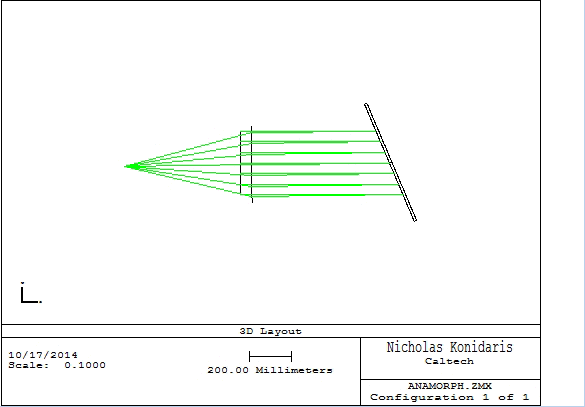
To illustrate the point, I’ve used zemax raytraces to create a number of videos that demonstrate the phenomenon and effect of anamorphism. As the web page loads, the videos should play in sync (if not, try reloading). The optical model shown in these videos represents a simplified spectrograph.
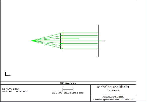
In the spectrograph, a single circular collimated beam illuminates a grating. The grating is either tilted or rotated (which varies with each frame of the movie), and the outgoing beam is fed into a perfect (paraxial) camera. The grating operates at a wavelength of 550 nm, with a ruling density of 280 line per millimeter operating in fifth order. The movie begins in the Littrow configuration ( and
and  ) and each frame of the movie increases the amount of grating tilt. As the tilt increases, the anamorphic factor increases to about 1.9.
The first frame shows the layout and ray traces. As the grating is tilted, the pupil on the camera increases in the dispersion direction. It is possible to measure the size of the beams on the screen with a ruler and compute the anamorphic factors.
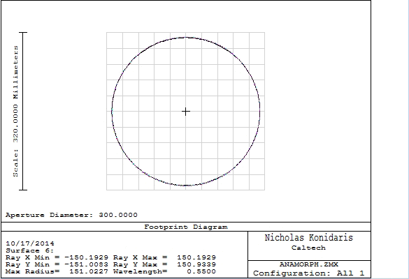
The second video shows a footprint diagram of the beam on the camera. The footprint diagram shows a grid for reference, a black circle tracing the camera mouth, and an ellipse expanding outward showing the rim of rays on the camera. You’ll notice some numbers on the bottom that compute the radius of the beam. The anamorphic factor can be computed by taking the Ray Max Radius and dividing it by 150. You’ll note that the final frame has a max radius of ~290 mm so the final anamorphic factor computed from this diagram is 1.933. Note the dispersion direction is perfectly aligned with the axis of pupil elongation.
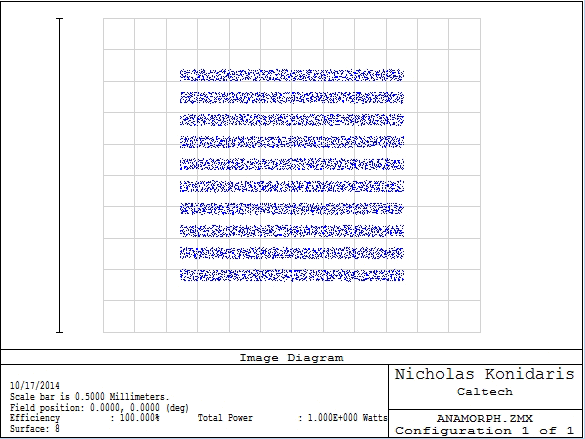
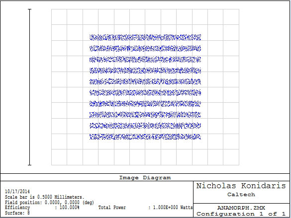
The third video shows an image on the detector. The image is comprised of dots where an individual ray hits the detector. The object is a series of horizontal lines, the envelope of the object is square. As the grating is tilted, the image of the object shrinks in the vertical direction (dispersion direction). The anamorphic advantage is that light from the object is concentrated into a smaller area as the anamorphic factor increases.
So we see here the pros and cons of tilt anamorphism. The anamorphic beam concentrates light from the object into fewer pixels, increasing the grasp of the instrument and decreasing the time to background limit. On the other hand, the beam presentation onto the camera is non circular and requires a larger and optically faster camera design.
β-angle rotation anamorphism
The angle is the angle projected along the line rulings in the grating. The effect of is described in the grating equation from above. How changes the pupil presentation and anamorphic factor is interesting and explored in this section.
In the previous section, I used zemax to raytrace beams through a simple spectrograph in order to observe the effect of tilting the grating in  from -23 degree to -60 degree. In this section I raytrace through the same spectrograph, but now rotate from 0 degree to 45 degree.
The three figures in this section are similar to those in the previous. The main difference is that the layout is rotated by 90 degree in order to see the effect of angle rotations. I won’t otherwise describe the figures again.
The result of angle rotations is surprising. Look at the footprint diagram. Recall that the vertical direction is the dispersion direction, notice that the footprint in the vertical direction does not change size. As a result, the length of the dispersed spectrum doesn’t shrink. Take a look at the static footprint diagram where is 45 degree. I have highlighted certain key features.

Now look at the movies. You’ll notice that pupil elongation angle is vertical for  and ends at almost 50 degree or so when is 45 degree. As the angle increases, the pupil in the spectral direction shrinks, while the pupil in the spatial direction stays the same. As a result, more pixels are required to capture the same spectrum in the spectral direction.

Conclusions
Bibliography
- Schweizer, F. 1979, PASP, 91, 149


 45 degree from the dispersion direction. Unlike tilt anamorphism,


